Alteryx Design Pattern: Nested headers in Excel files
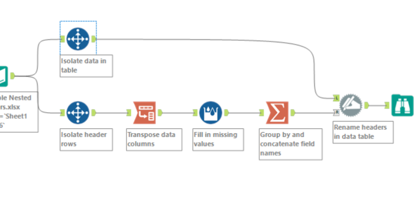
Are you a spreadsheet hero, but found that when you read the data into Alteryx the data doesn’t display as you would have expected?
This is probably because you are using nested headers in your spreadsheet. Nested headers are great visually as you don’t end up duplicating field names, however to work with data in Alteryx, you want you data to be tabular and unpivoted.
An example of a table with nested headers is shown below. In this example, the date appears in a row with merged cells for the monthly budget and actual amounts.

When this data is read into Alteryx, with the default settings the blank values above each monthly actual value are converted into generic field names (F1, F3, F5, F7), as Alteryx does not recognise merged cells.
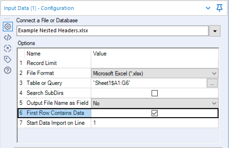
This design pattern will now walk through a process to convert these missing headers into the expected name so this we can use this for further analysis. By using a trick of actually forcing the data to use the generic field names, this is achieved by modifying the default configuration of the input data tool to assign standardised header names (F1 – F7), by stating that the first row of the table contains data.
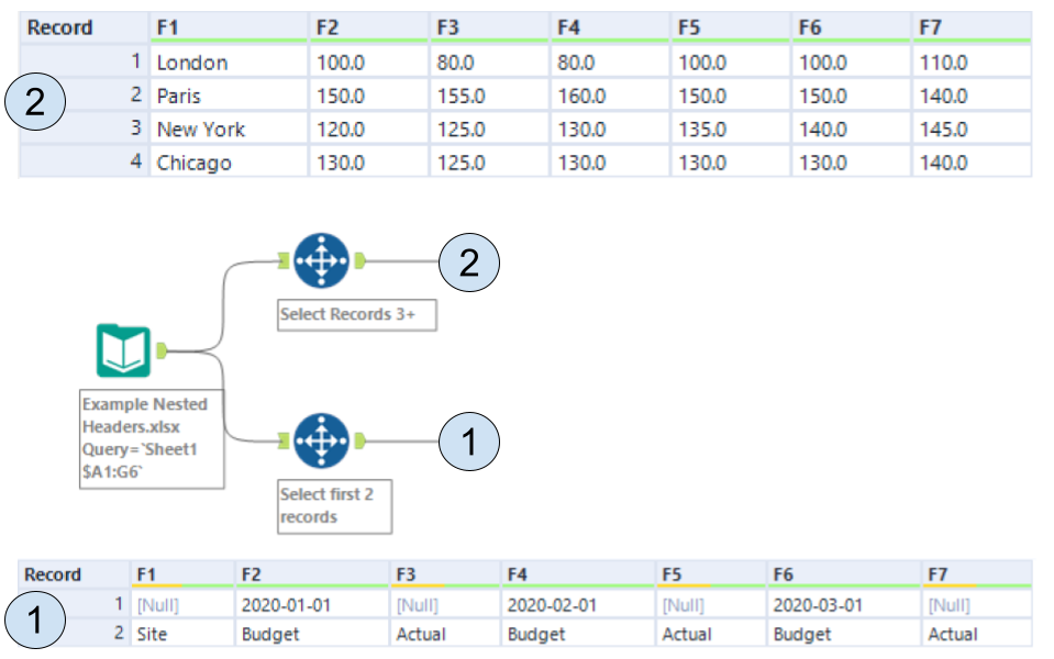
Once the input is forced to have standardised header names, we can split the workflow using select records, into two streams 1) to isolate the headers and 2) to isolate the data (N.B. Stream one is shown at the bottom as this makes it look neater when it feeds into the dynamic rename tool shown later).
With the input now split into these two streams the next part of this design pattern is focused on stream one, which reshapes the data and adds consistent field names.
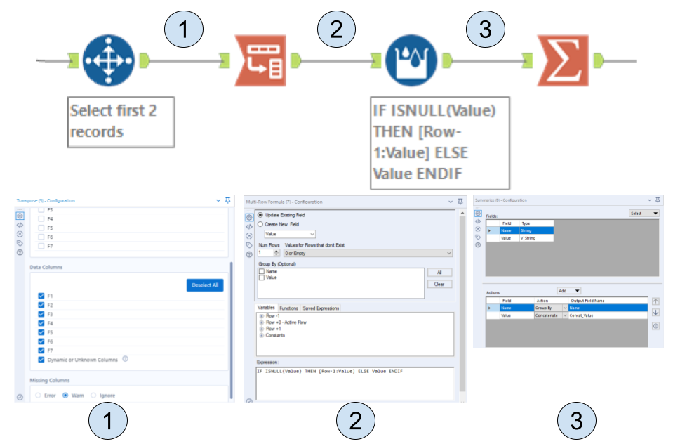
In these steps
- The transpose tool selects all columns as data columns which unpivots the data
- A multi-row formula is used to fill in the missing data
- A summarize tool to group by name and concatenating values joins together the date and budget or actual values of the nested headers
Once this is processed we can now use this stream in the workflow to rename the headers of the data that was isolated earlier. What the dynamic rename tool is doing here is similar to a find and replace, where the field names (F1 – F7) are replaced with newly created field names.
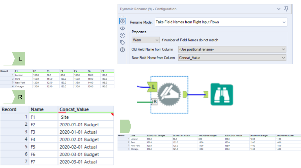
So this shows how a few tools can be used to modify merged and nested headers from Excel for processing as a table. If the layout of your Excel is different (i.e. more header rows or more columns merged) then the ultimate design pattern may need some tweaking, but hopefully this gives you the foundational tools to start building your own process.


